R Code Optimization IV: Practical Tools and Workflow

In the first post we established when and why to optimize, along with the three commandments that guide smart optimization decisions. The second post explored programming languages, clean code principles, and algorithm design. The third post tackled the heavy hitters: vectorization, parallelization, and memory management.

Now it’s time to bring theory into practice! This post focuses on the practical tools that transform optimization from guesswork into a systematic process. We’ll cover profiling to find bottlenecks, benchmarking to validate improvements, and the iterative workflow that ties everything together.

Requirements

This post uses several packages for profiling and benchmarking. Install them if you haven’t already:

install.packages(c("profvis", "microbenchmark", "bench"))

Profiling and Benchmarking

Profiling and benchmarking are methods to measure your code’s performance and help guide optimization decisions. The former helps identify low-performance hot-spots in your code, while the latter helps make informed choices between alternative implementations.

Profiling

Profiling helps analyze your code to understand where the execution time and RAM memory are spent, and will help you answer the question: Where should I start optimizing? Profilers break down code execution into function calls, highlighting potential bottlenecks

In R, the function utils::Rprof() is the default profiling tool. You can find a great explanation on this tool in the chapter Profiling R Code of the book R Programming for Data Science, by Roger D. Peng.

The function profvis::profvis() is a modern alternative that still uses Rprof() underneath, but generates a neat HTML widget to facilitate the visualization and interpretation of profiling data.

Let’s check how it works on the silly function f() shown below. It runs a correlation test between two large vectors generated randomly from a normal and a uniform distribution.

f <- function(n = 1e7){
  stats::cor.test(
    x = stats::rnorm(n = n), 
    y = stats::runif(n = n)
  )
}

To profile it with profvis() we just have to introduce our function into the argument expr. The argument rerun = TRUE is helpful to profile functions that might run too fast for the profiler.

profvis::profvis(
  expr = f(), 
  rerun = TRUE
  )

The Flame Graph shows the call stack of the profiled code. It indicates, from bottom to top, what functions are called by other functions, their run time, and memory allocated or deallocated. For example, on the lower right corner you can see how cor.test.default () calls the functions complete.cases and cor, and a gray block labelled <GC> wiht a negative memory number (indicating deallocated memory). These gray boxes show garbage collection calls, used for memory housekeeping.

The Data tab summarizes the profiling from top to bottom in a very intuitive way that highlights computational hot-spots in our code right away.

Even though profvis() is a very useful tool to guide software optimization, there are some limitations to be aware of: the memory usage values be unreliable due to R’s lazy memory management and the automated application of garbage collection, which can obscure memory allocations and deallocations.

If you wish to learn more, there are several profvis examples available in this vignette.

Other Profiling Tools

While profvis is the most popular and user-friendly profiling tool in R, there are several alternatives worth knowing about:

Another option leveraging Rprof() is the package proftools. It does not produce a neat html widget, but has extended plotting functionalities. It’s particularly useful when you need more customizable visualizations for specific use cases.

For memory-focused profiling, profmem and aprof provide detailed information about memory allocations in your code. These are particularly valuable when you’re trying to understand memory allocation patterns and reduce memory footprint, rather than just focusing on execution time.

xrprof is an experimental external profiler that can profile R code without modification. It’s useful for profiling code you can’t easily wrap in profvis() calls, though it requires more setup.

For most optimization workflows, profvis() is your best bet—it balances ease of use with actionable insights. But if you’re wrestling with tricky memory issues or need specialized profiling capabilities, these alternatives are worth exploring.

Benchmarking

Once we’ve profiled our code and identified a performance bottleneck worth addressing, it’s time to think about alternative implementations.

Remember the profiling example with f() above? It showed that stats::cor.test() accounts for a significant chunk of runtime and memory usage. We could try replacing it with the simpler stats::cor() to see if performance improves. But here’s the thing: how do we know if our “optimization” actually worked? Or if it made things worse?

This is where benchmarking comes in!

Benchmarking is the process of running alternative versions of code multiple times to rigorously compare their performance. It helps us make data-driven optimization decisions rather than relying on hunches or one-off timing measurements. The key difference from profiling: profiling shows you where the problems are, benchmarking shows you whether your solution works.

f_alt <- function(n = 1e7){
  stats::cor(
    x = stats::rnorm(n = n), 
    y = stats::runif(n = n)
  )
}

Benchmarking with microbenchmark

The microbenchmark package is the classic benchmarking tool in R. It runs each expression multiple times and provides statistical summaries of execution time.

Let’s compare different ways to extract a column from a data frame—a common operation with surprisingly variable performance:

library(microbenchmark)

df <- data.frame(
  x = stats::runif(n = 1e7)
)

microbenchmark::microbenchmark(
  df$x,
  df[["x"]],
  df[, "x"],
  dplyr::pull(df, x),
  times = 100
)

The output shows several timing statistics for each approach:

• min/max: Fastest and slowest execution times across all runs
• median: The middle value—often more reliable than mean for performance data
• mean: Average execution time
• lq/uq: Lower and upper quartiles (25th and 75th percentiles)

You’ll typically see that df$x and df[["x"]] are fastest, while df[, "x"] is slower due to additional overhead (it creates a single-column data frame rather than returning a vector). The dplyr::pull() approach adds function call overhead but might be worth it for code readability in a tidyverse-heavy codebase.

This kind of information helps you make informed trade-offs between code style, readability, and raw performance.

Benchmarking with bench

The bench package is a modern alternative to microbenchmark that provides additional insights, particularly around memory allocation.

library(bench)

benchmark_results <- bench::mark(
  df$x,
  df[["x"]],
  df[, "x"],
  dplyr::pull(df, x),
  iterations = 100,
  check = FALSE  # skip checking that all results are identical
)

benchmark_results

The bench::mark() output includes several valuable columns beyond just execution time:

• median/mean: Execution time statistics (same concept as microbenchmark)
• mem_alloc: Memory allocated during each operation
• n_gc: Number of garbage collection events triggered
• n_itr: Actual number of iterations performed

The memory allocation data is particularly enlightening! It reveals that df[, "x"] allocates a new object while df$x and df[["x"]] don’t. This explains both the performance difference and why the slower approach might cause issues with large data.

You can also visualize the results for a quick performance comparison:

plot(benchmark_results)

The plot shows the distribution of execution times, making it easy to spot which approaches are consistently fast versus which have high variability.

Benchmarking Best Practices

When benchmarking code, follow these principles to get meaningful results:

• Use realistic data: Test with data sizes and types that match your actual use case. Performance characteristics often change dramatically with scale—something fast with 1,000 rows might be slow with 1,000,000.

• Run sufficient iterations: Both microbenchmark and bench handle this automatically, but ensure you have enough repetitions for statistical confidence. The default (usually 100+) is typically adequate.

• Verify correctness first: Make sure your alternative implementations actually produce the same results! Use check = TRUE in bench::mark() or manually verify outputs. A fast but wrong solution is worthless.

• Consider memory alongside speed: The fastest approach isn’t always best if it consumes excessive memory or triggers frequent garbage collection. Look at execution time and memory metrics together.

• Benchmark the bottleneck, not everything: Focus your benchmarking on the specific code blocks identified during profiling. Don’t waste time optimizing operations that account for 1% of runtime.

• Test edge cases: If your code handles varying input sizes or types, benchmark with representative examples of each.

The Optimization Loop

Code optimization isn’t a one-time fix—it’s an iterative process. The diagram below illustrates the systematic workflow that brings together everything we’ve covered throughout this series:

Let’s walk through each step of this loop and see how it connects to the principles and techniques from the previous posts.

Step 1: Start with Working Code

Begin with code that’s correct and reasonably readable. This aligns perfectly with the First Commandment from Post I: “Thou shall not optimize thy code.”

Don’t optimize prematurely! Get your code working first, make sure it’s producing correct results, and ensure it’s reasonably clean. Trying to optimize broken or unclear code is a recipe for bugs and frustration.

Step 2: Identify the Need for Optimization

Before diving into optimization, ask yourself: Does this code actually need to be optimized?

Consider these factors:

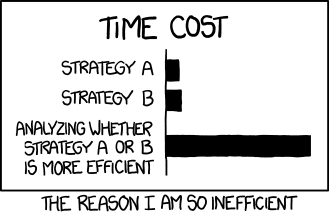
• Execution time: Is it genuinely slow enough to matter? Remember the XKCD efficiency comic—don’t spend hours optimizing code that saves seconds.

• Frequency: Does this code run once, or thousands of times? A function that runs once per day doesn’t need the same optimization effort as one that runs thousands of times per hour.

• Memory usage: Is it consuming excessive RAM? Causing crashes? Or is current memory usage acceptable?

• Scalability: Will this code need to handle much larger datasets in the future? Or is current scale the maximum you’ll encounter?

If the answers suggest your code is fast enough and efficient enough for its use case, stop here. The Second Commandment says “Thou shall make thy code simple”—and simple, working code that’s fast enough is already optimized!

Step 3: Profile to Find Bottlenecks

If optimization is genuinely needed, don’t guess where the problems are—measure!

Use profvis::profvis() to identify where execution time and memory are actually spent. The Pareto Principle applies here: typically 80% of your performance issues come from 20% of your code.

profvis::profvis({
  # Your code here
})

Focus your optimization efforts on the hot-spots revealed by profiling. Optimizing code that accounts for 2% of total runtime is rarely worth the complexity cost.

Step 4: Apply Optimization Techniques

Now bring in the techniques from throughout this series, starting with the lowest-hanging fruit:

From Post II:

• Is your code needlessly complex? Can better algorithm design help?
• Are you using appropriate data structures for your operations?
• Can cleaner code design actually improve performance while improving readability?

From Post III:

• Can you replace loops with vectorized operations?
• Is this task embarrassingly parallel and worth parallelizing?
• Are you managing memory efficiently, or creating unnecessary copies?

Apply the Third Commandment here: “Thou shall optimize wisely.” Make changes that offer significant performance gains without destroying code clarity. Sometimes the best optimization is choosing a better algorithm; sometimes it’s parallelization; sometimes it’s just removing unnecessary work.

Step 5: Benchmark Before and After

This step is critical—never skip benchmarking!

Use microbenchmark::microbenchmark() or bench::mark() to rigorously compare your original code with the optimized version:

bench::mark(
  original = original_function(data),
  optimized = optimized_function(data),
  iterations = 100
)

Benchmarking tells you:

• Did the optimization actually improve performance? (Sometimes “optimizations” make things worse!)
• How much faster is it? 10% improvement? 10x improvement?
• What’s the memory usage trade-off?
• Is the performance improvement consistent or variable?

If your optimization didn’t help, or made things worse, roll it back. Failed optimization attempts are learning opportunities, not wasted effort.

Step 6: Repeat or Stop

After benchmarking, you face a decision: continue optimizing or call it done?

Stop optimizing if:

• Performance is now acceptable for your actual use case
• Further optimization would significantly reduce code readability
• You’ve hit external bottlenecks (I/O, network, database queries) that code changes can’t fix
• You’re facing diminishing returns—spending hours to save milliseconds

Continue optimizing if:

• Performance still isn’t adequate for your needs
• Profiling reveals new bottlenecks after your changes (optimization can shift bottlenecks!)
• You’ve identified additional high-impact optimization opportunities
• You’re still in the “easy wins” phase where small changes yield big gains

Remember: optimization is about balance. A 90% performance improvement might be more than enough, even if theoretically you could squeeze out another 5% at the cost of code maintainability.

Putting It All Together: A Complete Example

Let’s see the optimization loop in action with a concrete example. Here’s some inefficient code that calculates rolling means on a vector:

# Original, inefficient version
rolling_mean_slow <- function(x, window = 3) {
  n <- length(x)
  result <- numeric(n)  # pre-allocation: good!

  for (i in window:n) {
    # Repeated subsetting and mean calculation: slow!
    result[i] <- mean(x[(i - window + 1):i])
  }

  return(result)
}

# Create test data
test_data <- runif(10000)

Step 1: Profile it

profvis::profvis({
  rolling_mean_slow(test_data)
})

Profiling reveals that the bottleneck is the repeated subsetting x[(i - window + 1):i] and the mean() function calls inside the loop. Each iteration creates a new vector subset and calculates its mean—lots of unnecessary overhead!

Step 2: Optimize using vectorization

From Post III, we know that R has highly optimized functions for common operations. The stats::filter() function is specifically designed for this kind of rolling calculation:

# Optimized version using vectorization
rolling_mean_fast <- function(x, window = 3) {
  stats::filter(x, rep(1/window, window), sides = 1)
}

This version leverages R’s built-in, compiled C code for filtering operations. No loops in R-land, no repeated subsetting—just a single vectorized operation.

Step 3: Benchmark the results

bench::mark(
  slow = rolling_mean_slow(test_data),
  fast = rolling_mean_fast(test_data),
  iterations = 100,
  check = FALSE
)

The optimized version is typically 10-50x faster, depending on data size and window size. And here’s the beautiful part: it’s not just faster, it’s also simpler and more readable. The best optimizations often are!

This is the optimization loop in practice: profile, optimize the bottleneck, benchmark to confirm improvement, and move on.

Wrapping Up This Series

We’ve covered substantial ground across these four posts:

Post I: Foundations and Principles The three commandments, dimensions of code efficiency, when to optimize (and when not to), and the Pareto Principle.

Post II: Language, Design, and Readability Compiled vs interpreted languages, clean code principles, algorithm design, and data structures.

Post III: Hardware Utilization Vectorization (SIMD and semantic), parallelization (explicit and implicit), and memory management strategies.

Post IV: Practical Tools and Workflow (this post) Profiling with profvis, benchmarking with microbenchmark and bench, and the iterative optimization loop.

The Core Message

Code optimization is fundamentally about balance and trade-offs:

• Balance between computational performance and code readability
• Trade-offs between execution speed and memory usage
• Balance between optimization effort and practical benefit

The goal isn’t writing the absolute fastest code possible—it’s writing code that’s fast enough, maintainable, correct, and sustainable. Clean, well-designed code that runs adequately fast is infinitely more valuable than unreadable code that’s microseconds faster.

Follow the three commandments:

1. Don’t optimize prematurely
2. Optimize for simplicity and readability first
3. When performance optimization is needed, do it wisely

Use profiling to find real bottlenecks, apply appropriate optimization techniques from the toolkit we’ve covered, benchmark rigorously to validate improvements, and know when to stop.

Now you have the principles, the techniques, and the tools. Go forth and optimize wisely!

Additional Resources

Want to dive deeper into R optimization? These resources are excellent:

• Advanced R by Hadley Wickham: Essential reading, particularly Chapter 24 on Improving Performance.

• Efficient R Programming by Colin Gillespie and Robin Lovelace: Comprehensive coverage of optimization topics with practical examples.

• The Art of R Programming by Norman Matloff: Chapter 14 on performance is somewhat dated but offers valuable insights on speed-memory trade-offs.

• R Programming for Data Science by Roger Peng: The chapter on profiling is an excellent practical introduction.

• Best Coding Practices for R: Chapters 10-12 cover memory management techniques in detail.

Thanks for sticking with me through all four posts! I hope you found them helpful and that they improve both the quality and efficiency of your R code.

Happy optimizing!