A Gentle Intro to Dynamic Time Warping
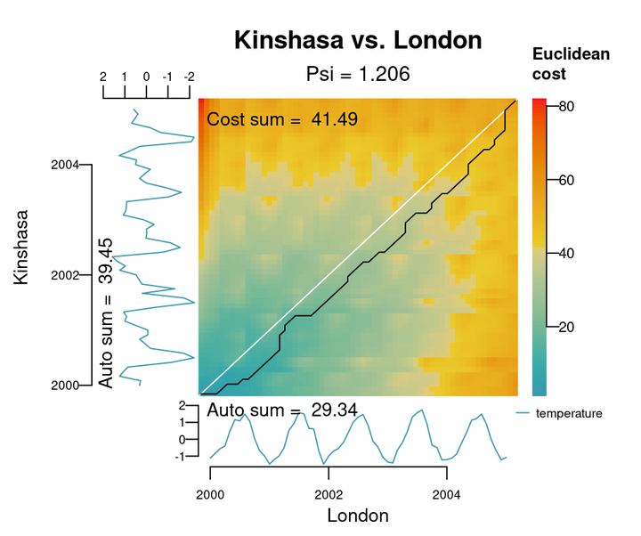 Graph by Blas M. Benito
Summary
This post provides a gentle conceptual introduction to Dynamic Time Warping (DTW), a method to compare time series of different lengths that has found its way into our daily lives. It starts with a very general introduction to the comparison of time series, follows with a bit of history about its development and a step-by-step breakdown, to finalize with a summary of its real-world applications.
Comparing Time Series
Time series comparison is a critical task in many fields, such as environmental monitoring, finance, and healthcare. The goal is often to quantify similarities or differences between pairs of time series to gain insights into how the data is structured and identify meaningful patterns.
For example, the data below shows time series representing the same phenomenon in three different places and time ranges: a and b have 30 synchronized observations, while c has 20 observations from a different year.
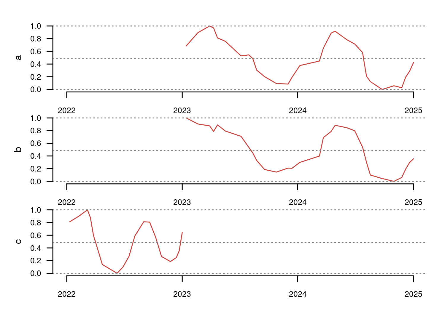
There are several options to compare a and b directly, such as assessing their correlation (0.955), or computing the sum of Euclidean distances between their respective samples (2.021).
This comparison approach is named lock-step (also known as inelastic comparison), and works best when the time series represent phenomena with relatively similar shapes and are aligned in time and frequency, as it is the case with a and b.
Comparing c with a and/or b is a completely different task though, exactly the one
Dynamic Time Warping was designed to address.
Now it would make sense to explain right away what dynamic time warping is and how it works, but there’s a bit of history to explore first.
A Bit of History
Dynamic Time Warping (DTW) might sound like a modern high-tech buzzword, but its roots go way back—older than me (gen X guy here!). This powerful method was first developed in the pioneering days of speech recognition. The earliest reference I uncovered is from Shearme and Leach’s 1968 paper, Some experiments with a simple word recognition system, published by the Joint Speech Research Unit in the UK.
These foundational ideas were later expanded upon by Sakoe and Chiba in their seminal 1971 paper, A Dynamic Programming Approach to Continuous Speech Recognition, often regarded as the definitive starting point for modern DTW applications.
From there, DTW has found applications in diverse fields relying on time-dependent data, such as medical sciences, sports analytics, astronomy, econometrics, robotics, epidemiology, and many others.
Ok, let’s stop wandering in time, and go back to the meat in this post.
What is Dynamic Time Warping?
Dynamic Time Warping is a method to compare univariate or multivariate time series of different length, timing, and/or shape. To do so, DTW stretches or compresses parts of the time series (hence warping) until it finds the alignment that minimizes their overall differences. Think of it as a way to match the rhythm of two songs even if one plays faster than the other.
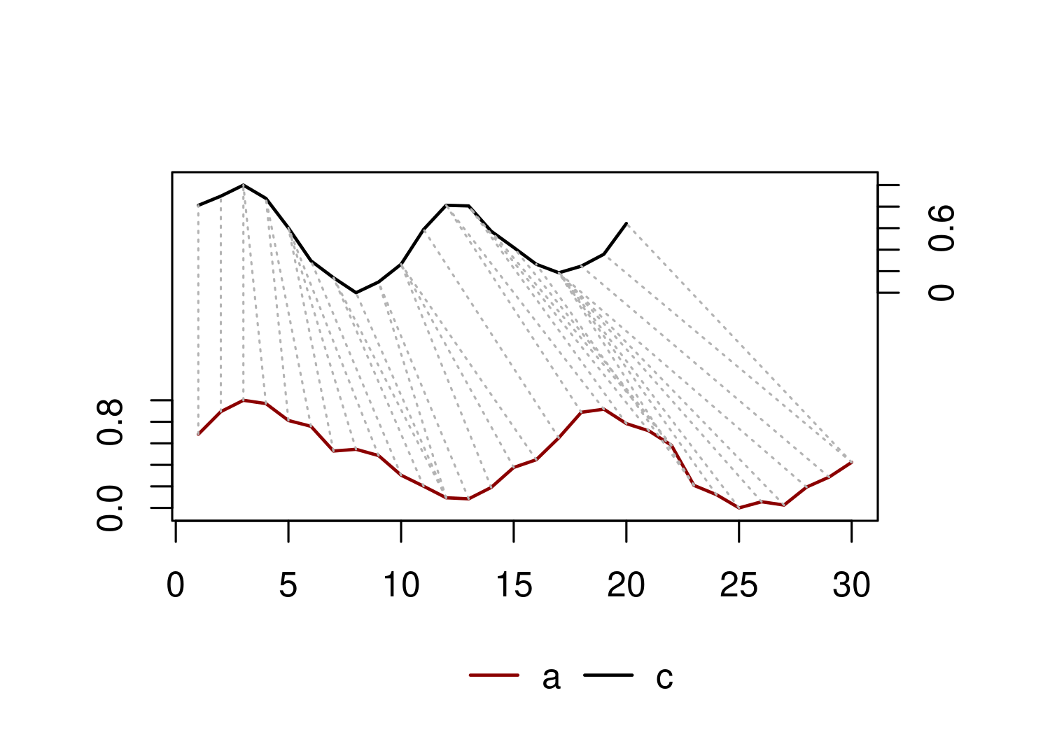
The figure below represents a dynamic time warping solution for the time series c and a. Notice how each sample in one time series matches one or several samples from the other. These matches are optimized to minimize the sum of distances between the samples they connect (3.285 in this case). Any other combination of matches would result in a higher sum of distances.
In dynamic time warping, the actual warping happens when a sample in one time series is matched with two or more samples from the other, independently of their observation times. The figure below identifies one of these instances with blue bubbles. The sample 10 of c (upper blue bubble), with date 2022-07-16, is matched with the samples 14 to 16 of a (lower bubble), with dates 2023-12-13 to 2024-03-09. This matching structure represents a time compression in a for the range of involved dates.
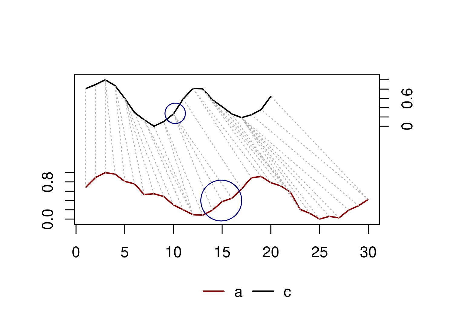
This ability to warp time makes DTW incredibly useful for analyzing time series that are similar in shape but don’t have the same length or are not fully synchronized.
The next section delves into the computational steps of DTW.
DTW Step by Step
Time series comparison via Dynamic Time Warping (DTW) involves several key steps:
- Detrending and z-score normalization of the time series.
- Computation of the distance matrix between all pairs of samples.
- Computation of a cost matrix from the distance matrix.
- Finding the least-cost path within the cost matrix.
- Computation of a similarity metric based on the least-cost path.
Detrending and Z-score Normalization
DTW is highly sensitive to differences in trends and ranges between time series (see the Pitfalls section). To address this, detrending and z-score normalization are important preprocessing steps. The former removes any upwards or downwards trend in the time series, while the later scales the time series values to a mean of zero and a standard deviation of one.
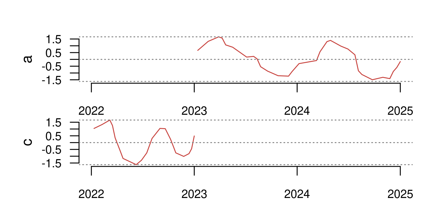
In this example, the time series a and c already have matching ranges, so normalization is not strictly necessary. For demonstration purposes, however, the figure below shows them normalized using z-score scaling:
Distance Matrix
This step involves computing the distance matrix, which contains pairwise distances between all combinations of samples in the two time series.
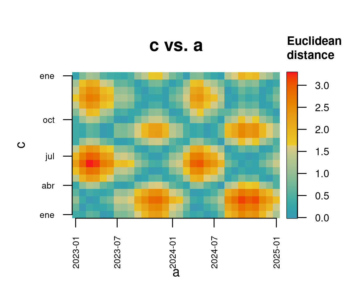
Choosing an appropriate distance metric is crucial. While Euclidean distance works well in many cases, other metrics may be more suitable depending on the data.
Cost Matrix
The cost matrix is derived from the distance matrix by accumulating distances recursively, neighbor to neighbor, from the starting corner (lower-left) to the ending one (upper-right).
Different rules for cell neighborhood determine how these costs propagate:
- Orthogonal only: Accumulation occurs in the x and y directions only, ignoring diagonals.
- Orthogonal and diagonal: Diagonal movements are also considered, typically weighted by a factor of
√2(1.414) to balance with orthogonal movements.
The figure below illustrates the cost matrix with both orthogonal and diagonal paths.
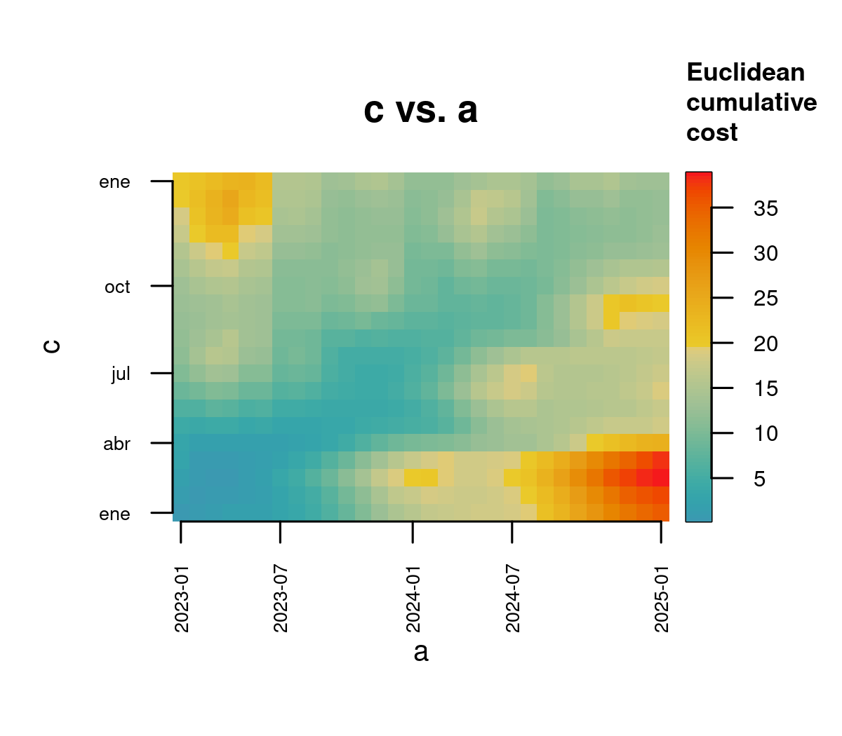
The result of the cost matrix is similar to the topographic map of a valley, in which the value of each cell represents the slope we have to overcome to walk through it.
Now that we have a valley, let’s go create a river!
Least-cost Path
This is the step where the actual time warping happens!
The least-cost path minimizes the total cost from the start to the end of the cost matrix, aligning the time series optimally.
The algorithm building the least-cost path starts on the upper right corner of the cost matrix, and recursively selects the next neighbor with the lowest cumulative cost to build the least-cost path step by step. This process is similar to letting a river find its shortest path way down a valley.
The figure below shows the least-cost path (black line). Deviations from the diagonal represent adjustments made to align the time series.

Similarity Metric
Finally, DTW produces a similarity metric based on the least-cost path. The simplest approach is to sum the distances of all points along the path.
For this example, the total cost is 7.588. However, when comparing time series of varying lengths, normalization is often useful. Common options include:
- Sum of lengths: Normalize by the combined lengths of the time series, e.g.,
Normalized Cost = Total Cost / (Length(a) + Length(c)). Foraandc, this would be 0.152. - Auto-sum of distances: Normalize by the sum of distances between adjacent samples in each series, as in
Normalized Cost = Total Cost / (Auto-sum(a) + Auto-sum(c)). Foraandc, this results in 0.358.
These normalized metrics allow comparisons across datasets with varying characteristics.
Real World Applications
Dynamic Time Warping is a well-studied topic in academic community, with more than 86k research articles listed in Google Scholar. However, the real-world impact of an academic concept often differs from its academic popularity. Examining DTW-related patents provides a clearer view of its practical applications.
The United States Patent and Trademark Office includes the class 704/241 specifically for “Dynamic Time Warping Patents”. Similarly, the Cooperative Patent Classification includes the classification (G10L 15/12) with the title “Speech recognition using dynamic programming techniques, e.g. dynamic time warping (DTW)”.
Using the European Patent Office search tool Spacenet for “Dynamic Time Warping” returns approximately 12.000 results. Google Patents reports over 35.000 results.
While patents illustrate the technical implementation of DTW, uncovering its application in company blogs, wikis, or manuals is more challenging. Nonetheless, a few compelling examples demonstrate DTW’s real-world utility.
Media and Entertainment
Closed caption alignment is perhaps the most pervasive yet invisible application of DTW. Companies like Netflix and Microsoft use DTW to synchronize subtitles with soundtracks in movies, TV shows, and video games, ensuring an accurate match regardless of pacing or timing inconsistencies.
Wearables and Fitness Devices
Many wearables employ DTW to classify user activities by aligning accelerometer and gyroscope data with predefined templates. For example, Goertek’s Comma 2 smart ring presented in January 2025 uses DTW to recognize user movements. Another creative example is the Wave MIDI controller ring, patented by Genki. This device applies DTW with a nearest-neighbor classifier to analyze hand movements and trigger musical effects.
Biomechanics
In biomechanics, DTW helps analyze movement patterns and detect anomalies. For instance, the software Sift by HAS Motion uses DTW to compare large datasets of movement traces and identify deviations. Similarly, the OrthoLoad processes load measurements on joint implants using DTW to analyze patterns and identify irregularities.
Industrial Applications
DTW is also used in manufacturing to monitor machinery health. Toshiba’s LAMTSS technology applies DTW to noise and motion data from manufacturing equipment, helping detect and predict operational failures before they occur.
These examples highlight the versatility and practical relevance of DTW, spanning industries from entertainment to biomechanics and industrial maintenance. Its ability to adapt to diverse time series challenges underscores its value in real-world problem-solving.
Closing Thoughts
Dynamic Time Warping exemplifies how a sophisticated algorithm, initially developed for niche applications, has evolved into a versatile tool with real-world significance. From aligning movie subtitles to monitoring machinery health, DTW bridges the gap between academic theory and practical innovation. Its ability to adapt to various industries highlights the importance of robust time series analysis techniques, and further cements its place in both research and applied fields.